Introduction

In A Walk Though of Accessing Financial Statements with XBRL in R - Part 1, we showed how to use R to extract Apple financial statement data from the SEC Edgar website. This would be a cumbersome process to scale across sectors, but works well for a single company. In Tracking R&D spending by 700 Listed US Pharma Companies - Part 2, we went a step further to collect data from over 700 listed pharmaceutical stocks from the free at the time Financial Modeling Prep API. We learned that Financial Modeling Prep has subsequently gone to a paid model, but there is a new R package called fmpapi expected imminently on CRAN, which looks exciting and possibly making worthy of subscribing for $14/month. The drawback with both of these methods is that queries are constrained to the full financial statements of a given company. What if we could look datapoint-by-datapoint across all companies and time periods?

In this series, we will explore another option for extracting large amounts of financial statement data via XBRL from secdatabase.com, which also maintains a paid UI for 150 institutional clients with access to all Edgar filings (not just the 10-K and 10-Q as in the database we will use here). For the database, secdatabase.com offers two plans, one with free access to all 10-K and 10-Q filings since 2009, but with a lag and also not including full text search. We are told that the paid option will include real time filings as well as full text search. The database is over 20GB, and searches are conducted using AWS Athena, with charges we found to be nominal. The best thing about this method in comparison to the previous methods used, is that the data is one large pool, and hence, any single data point can be extracted for any or all companies, sectors or time periods. Response times are also instantaneous, instead of minutes or hours using the other sources when data across a large number of companies was needed.

There are multiple objectives for this series in addition to our ongoing explorations of XBRL. First, we will (1) show how to set up a database to be queried from AWS Athena, (2) demonstrate the RStudio functionality for connecting to databases, (3) to take advantage of the opportunity to improve our SQL while exploring XBRL, and (4), to better understand the hierarchy of the XBRL taxonomy. For those who already know how to set up and query a database from RStudio, the this first post may be too much detail, so skip to the next posts in the index below. However, for those who haven’t done this before, posts which don’t assume any prior experience can be very helpful.

Links to other post in this series: TBA

Setting Up secdatabase.com in AWS Athena

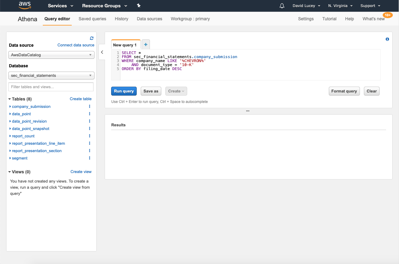
When we first looked at the instructions to set up SEC XBRL Financial Statement Dataset, we were lost, but a short conversation with a secdatabaserep solved everything. Steps 1. and 2. were very straightforward. Log into AWS, navigate to Athena and copy/paste the query “CREATE DATABASE sec_financial_statements;” (no quotes) into the “New Query 1” tab and run the query, which will establish the link to the source in the “AWSDataCatalog” from within Athena. The second part is easy, but at first, was confusing for us without help from the rep. Navigate to the “sql” folder in SEC XBRL Financial Statement Dataset, and copy/paste the queries one-by-one (except for the last one which is already done) into new query tabs then run. Each of these queries will create a table within “sec_financial_database”. After running, each these tables, along with their fields, will be visible within the AWS “Tables” tab, and ultimately, from the “Connections” pane in RStudio.

AWS Athena sec_financial_statements Database

After this, navigate to S3, set up a bucket for this project, and within the bucket, create a folder to store queries and any materialized data. We have called our bucket “secdatabase-test” and our folder “experiment”, which will be used to make the connection. After a week of practicing making queries, we have run up about \(1.50 of Athena charges and `\)0.01 onS3`, because we have mostly returned only small summary tables. But be careful, it would be easy to fill up S3 and run up more meaningful charges materializing large queries with a 20GB+ data set.

Setting Up Connection in RStudio

There are several ways of connecting to Athena in R. Although we didn’t explore too much, we had a few challenges installing with ODBC, and RAthena uses our favorite data.table in order to improve efficiency of communication with AWS, so that seemed like a natural choice. RAthena uses the Python boto3 library to connect to AWS, and hence needs reticulate and a miniconda environment with boto3 installed. It also offers a function called install_boto() to manage this process if you don’t currently have miniconda installed, but we chose to pip install boto3 in the existing miniconda environment on our machine. In the chunk below, we specify the miniconda environment with boto3 for this project.

# Choose Python 3.7 miniconda
reticulate::use_condaenv(
  condaenv = "r-reticulate",
  required = TRUE
  )

In addition to using data.table to handle interactions with AWS, we prefer to use data.table for all of our data wrangling, and RAthena allows us to chose to have the SQL query return a data.table.

RAthena_options(file_parser = "data.table")

The Athena Simba Driver has to be installed from Simba Athena ODBC Driver with SQL Connector 1.0.6 Installation and Configuration Guide. We were able to accomplish this with the instructions given by the link. In order for the connection from RStudio to find the Simba Driver, the following lines must be saved in the odbc.ini and odbcinst.ini text files, which you will find in usr/local/etc on Mac. Another way to find these is to search “odbc” with Spotlight.

Save in file odbc.ini:

[Simba Athena ODBC Driver]
Driver = /Library/simba/athenaodbc/lib/libathenaodbc_sbu.dylib

Save in file odbcinst.ini:

[Simba Athena ODBC Driver]
Driver=/Library/simba/athenaodbc/lib/libathenaodbc_sbu.dylib

A good way to check if that the ODBC driver has been installed and linked is is here:

sort(unique(odbc::odbcListDrivers()[[1]]))

[1] "MySQL Driver"             "ODBC Drivers"            
[3] "PostgreSQL Driver"        "Simba Athena ODBC Driver"
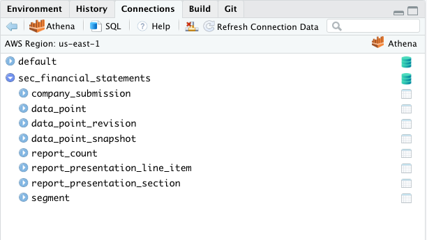
[5] "SQLite Driver"           

Lastly, the code to set up the connection object with our AWS Access Key ID and AWS Secret Access Key is shown below. We have used the keyring package to hide our credentials as our code will be posted on Github, but any other method is also fine. The driver is straightforward as RAthena::athena(). At first, we were unsure what to set for the schema and used “default”, as that was one of the options in our Athena Query Editor page, but we later learned that the correct choice was “sec_financial_statements”. When this is used, the database and all the tables can be navigated from RStudio’s “Connections” pane as shown below (almost as if they were regular data.frames in the global environment). This is not exactly the case because the data hasn’t been “materialized”, but it is helpful in visualizing the fields in each table and traversing the database.

con <- dbConnect(RAthena::athena(),
                aws_access_key_id=keyring::key_get('AWS_ACCESS_KEY_ID'),
                aws_secret_access_key=keyring::key_get('AWS_SECRET_ACCESS_KEY'),
                schema_name = "sec_financial_statements",
                s3_staging_dir='s3://secdatabase-test/experiment/',
                region_name='us-east-1')

Once the connection is established, it can be checked with the regular DBI functions.

DBI::dbGetInfo(con)

$profile_name
NULL

$s3_staging
[1] "s3://secdatabase-test/experiment/"

$dbms.name
[1] "sec_financial_statements"

$work_group
[1] "primary"

$poll_interval
NULL

$encryption_option
NULL

$kms_key
NULL

$expiration
NULL

$keyboard_interrupt
[1] TRUE

$region_name
[1] "us-east-1"

$boto3
[1] "1.14.50"

$RAthena
[1] "1.10.0"

Structure of secdatabase

A summary of the tables we just set up in the “sec_financial_statements” database can be seen as shown with the “Connections” pane in RStudio. At the right, the icons can be used to view a sample of rows in that table almost like an ordinary spreadsheet without moving the data into RStudio.

RStudio Connections Pane

Fields in the “company_submission” table can be also be seen with dbListFields() below. Each company has a “cik” identifier and each filing has an common “accession_number_int” key. Other identifier information about the company like the SIC code (“assigned_sic”), the document_type (ie: 10-K or 10-Q), filing date and period along with other aspects of the company. We found ourselves using this table to filter on “10-K” OR “10-Q”, then joining with the “data_point_snapshot” or the “report_presentation_line_item” on “accession_number_int” most commonly.

dbListFields(con, "sec_financial_statements.company_submission")

 [1] "accession_number_int"          "accession_number"             
 [3] "cik"                           "company_name"                 
 [5] "filing_date"                   "document_type"                
 [7] "document_period_end_date"      "current_fiscal_year_end_date" 
 [9] "document_fiscal_year_focus"    "document_fiscal_period_focus" 
[11] "current_fiscal_year_end_month" "amendment_flag"               
[13] "assigned_sic"                  "irs_number"                   
[15] "state_of_incorporation"        "mailing_address_street1"      
[17] "mailing_address_street2"       "mailing_address_city"         
[19] "mailing_address_state"         "mailing_address_zip"          
[21] "business_address_street1"      "business_address_street2"     
[23] "business_address_city"         "business_address_state"       
[25] "business_address_zip"          "mailing_phone_number"         
[27] "business_phone_number"        

Another way to look at and interact with a table is using dplyr’s tbl() function as shown below. Our original intention was to use this method, but some functions we hoped to use (ie: regular expressions for filtering rows) are apparently not yet implemented. Instead, we shifted to using mostly RStudio’s SQL chunks, but dplyr has obvious appeal, because it is so seamless with a regular RStudio work flow, accept for the data.frame has to be materialized to bring the data into memory.

company_submission <- dplyr::tbl(con, "company_submission")
head(company_submission, 10)

# Source:   lazy query [?? x 27]
# Database: Athena 1.14.50 [us-east-1/sec_financial_statements]
   accession_numbe… accession_number   cik company_name filing_date
            <int64> <chr>            <int> <chr>        <date>     
 1     217814000056 0000002178-14-0…  2178 ADAMS RESOU… 2014-08-11 
 2     296917000031 0000002969-17-0…  2969 AIR PRODUCT… 2017-08-01 
 3     296917000039 0000002969-17-0…  2969 AIR PRODUCT… 2017-11-16 
 4     296918000014 0000002969-18-0…  2969 AIR PRODUCT… 2018-01-26 
 5     349916000040 0000003499-16-0…  3499 ALEXANDERS … 2016-05-02 
 6     357012000143 0000003570-12-0…  3570 CHENIERE EN… 2012-11-02 
 7     357013000036 0000003570-13-0…  3570 CHENIERE EN… 2013-02-22 
 8     357013000161 0000003570-13-0…  3570 CHENIERE EN… 2013-08-02 
 9     418714000008 0000004187-14-0…  4187 INDUSTRIAL … 2014-01-10 
10     418715000010 0000004187-15-0…  4187 INDUSTRIAL … 2015-08-14 
# … with 22 more variables: document_type <chr>,
#   document_period_end_date <date>, current_fiscal_year_end_date <chr>,
#   document_fiscal_year_focus <int>, document_fiscal_period_focus <chr>,
#   current_fiscal_year_end_month <int>, amendment_flag <lgl>,
#   assigned_sic <int>, irs_number <chr>, state_of_incorporation <chr>,
#   mailing_address_street1 <chr>, mailing_address_street2 <chr>,
#   mailing_address_city <chr>, mailing_address_state <chr>,
#   mailing_address_zip <chr>, business_address_street1 <chr>,
#   business_address_street2 <chr>, business_address_city <chr>,
#   business_address_state <chr>, business_address_zip <chr>,
#   mailing_phone_number <chr>, business_phone_number <chr>

As mentioned above, the “data_point_snapshot” (not to be confused with “data_point” table) is the primary table storing the final financial statement elements and values. As filings come in, all data points are all added to the “data_point” table by date with the same “accession_number_int” (the filing key identifier), whether or not they are the same as the previous version. If a data point in a particular filing is revised, it is added as another row in the “data_point” table, and the value recorded for that “datapoint_id” and associated “datapoint_name” is updated to the new value in the “data_point_snapshot” table and also to the “data_point_revision” table. Hence, “data_point” may have multiple values for the same datapoint_name and datapoint_id, and “data_point_snapshot” should have the just the one final value.

dbListFields(con, "sec_financial_statements.data_point_snapshot")

 [1] "cik"                  "accession_number_int" "filing_date"         
 [4] "datapoint_id"         "datapoint_name"       "version"             
 [7] "segment_label"        "segment_hash"         "start_date"          
[10] "end_date"             "period_month"         "string_value"        
[13] "numeric_value"        "decimals"             "unit"                
[16] "footnotes"            "revision_num"        

The “report_presentation_section” has a field called the “statement_type”, which can be used to filter for the type of statement (“Income Statement,”Balance Sheet“, etc), then join with”accession_number_int" to get only the data points for that company and the chosen statement.

dbListFields(con, "sec_financial_statements.report_presentation_section")

[1] "cik"                        "filing_date"               
[3] "accession_number_int"       "section_sequence_id"       
[5] "statement_type"             "report_section_description"

The next level down is the “report_presentation_line_item” table which allows to drill down into a parent_datapoint_name or datapoint_name within a given table. A datapoint_name might be “Revenue” or “NetProfitLoss”, or any other XBRL line-item financial statement identifier.

dbListFields(con, "sec_financial_statements.report_presentation_line_item")

[1] "accession_number_int"  "section_sequence_id"   "line_item_sequence"   
[4] "parent_datapoint_name" "datapoint_name"        "preferred_label_role" 
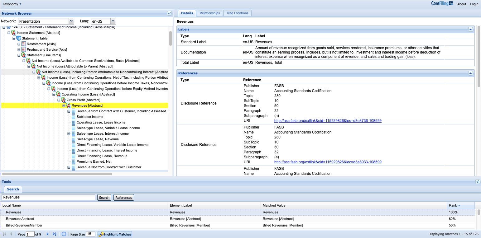
[7] "datapoint_label"       "datapoint_id"         

XBRL is governed by a complicated taxonomy, which has the as reported reported financial statement at the top of the hierarchy, then nested levels down to “facts”, which are root string or numeric elements or components of reported elements. One useful tool for navigating the XBRL Taxonomy is Corefiling shown in the view below. The “Revenues” datapoint_name or label is shown nested 10 levels down from the “Income Statement Abstract”, which itself is a child of the “Statement of Net Income (Including Gross Margin)” presentation. We would like to understand better how to navigate this complicated hierarchy, but so far have struggled to find information or figured out to decode it ourselves. Although secdatabase offers the fastest, most efficient way to treat the Edgar as one fluid data set, it is also an added layer of complexity because the nesting incumbent in XBRL has been flattened into tables with line-items which may be parents or children of other line-items.

Corefiling

Conclusion

As we will show in subsequent posts, multiple tables will generally have to be joined in order to pinpoint desired elements. As we will show, we discovered that it is not trivial to target the single desired data point or series of data points. Most of the literature that we could find about XBRL was from the perspective of financial statement preparers, and very little discussed how an investor would go about finding data in this complicated structure in order to conduct an analysis. Exploring XBRL in secdatabase in our next post is going to be much more difficult.